01. 대규모 모델 학습의 어려움
2012년 ImageNet Competition에서 부터는 딥러닝을 사용한 방법들이 우수한 성적을 거두고 있다. layer를 적절히 많이 쌓을 수록 오분류이 줄어들고 더 좋은 성과를 내는 것을 확일 할 수 있다. 하지만 딥러닝 학습을 위해서는 생각해 보아야 할 문제들이 존재한다. 그것이 무엇인지 살펴보자
1. 데이터를 얼마나 모아야 하는 것일까?
- 딥런닝을 위해서는 질좋은 많은 양의 데이터가 필요하다.
- 위의 그림에서도 알 수 있듯이 질좋은 데이터를 가지고 딥러닝 학습을 했는데 좋은 결과를 얻지 못했다면 결국 더 많은 양의 데이터를 가지고 학습을 해야한다는 것을 알 수 있다.
2. 모델을 학습시키는데에 들어가는 비용
- GPT-3 모델의 parameter개수 : 1759억개
- GPT-3를 학습시킬때 자동차로 달까지 왕복하는 것과 비슷한 수준의 온실가스가 발생했을 거이라고 추청
- 학습시키는데 최고 1000만 달러가 필요한 것으로 추측
➞ 이러한 고민들에서 질좋은 많은 양의 데이터도 없고 모델을 학습시키는데 필요한 충분한 비용도 없다면 어떻게 해야 딥러닝 모델을 사용할 수 있을까? 라는 고민에서 시작된 것이 Transfer Learning이다.
02. Transfer Learning
1. 처음부터 학습하기 vs. 학습된 모델 이용하기
우리가 특정한 모델을 사용하고 싶을 때 처음부터 우리가 학습시킨 모델을 사용하는 것이 좋을 까? 이미 누군가가 학습시킨 모델을 사용하는 것이 좋을 까? 만약 우리가 모델을 처음부터 학습 시킨다면 파라미터 초기화, 학습 등 모든 과정의 코드를 작성하고 실행해야한다. 또한 loss값을 확인하면서 성능이 좋아질 때까지 모델 학습을 진행해야한다. 사실 생각해보면 모델은 잘 학습시킨 파라미터 값을 저장해 놓고 있다. 그렇다면 누군가가 이미 대용량의 질좋은 모델을 가지고 학습을 시켜놓았다면 굳이 우리가 모델을 다시 학습 시킬 필요는 없다. 우리는 그냥 그 모델의 파라미터를 가져다가 사용하면 된다. 이렇게 미리 학습된 모델을 Pre-training Model이라 하고 Pre-training Model을 사용해 학습한 것을 Transfer Learning이라고 한다.
- Training From Scratch : training을 처음부터 한 모델
- Transfer Learning : Pre-training Model을 사용하는 것
2. Transfer Learning의 효관
- Pre-trained된 모델을 사용하여 새로운 모델을 만들기 때문에 학습이 빠르고 예측 능열을 더 높일 수 있다.
- 복잡한 모델일 수록 학습시키기 어렵다는 단점을 해결 할 수 있다.
- 학습에 들어가는 연산 비용을 절감할 수 있다.
- UGG, ResNet, Inception도 pre-trained된 모델을 가지고 사용할 수 있다.
03. Transfer Learning의 적용
1. Layer 별 featuer Learning의 차이
- input과 가까운 쪽으로 가면 간단한 feature를 학습한다.
- inpurt과 멀어질수록 더 복잡한, 복합적인 feature를 학습한다.
- Domain Specific : 도메인 특화
- Domain : 내가 분석하고자 하는 것
2. VGG16 모델 학습하기
- 16 ➞ 연산이 필요한 layer의 수
- output과 가까워 질수록 실질적으로 영향을 주는 featrue들을 학습한다.
- 데이터셋의 사이즈가 충분히 크다면
- VGG16모델 전체를 학습하면 된다.
- 데이터셋의 사이즈가 작다면
- Feature Extractor의 부분을 Freeze한다.
- 내가 가지고 있는 데이터에 직접적으로 영향을 주는 부분만 학습을 시키자!!
- 나머지는 pre-trained된 값을 가져온다.
- 데이터가 많지도 작지도 않다면
- training하는 layer의 영역을 조금씩 늘려간다.
- 시행착오를 통해 적절한 학습 정도를 찾아야한다.
- pretraing된 데이터와 내가 가진 data의 Domain이 얼마나 유사한지를 본다.
- 내가 가지고 있는 데이터가 어느정도인지 파악해본다.
코드 실습
- ResNet50 transfer learning
import os
import tensorflow as tf
import matplotlib.pyplot as plt

# 각각의 클래스에 해당하는 이미지의 개수를 알아보기 위해, 실습 데이터의 클래스마다 파일 경로를 변수로 정의
train_dir='aiffel/cifar_10_small/train'
test_dir='aiffel/cifar_10_small/test'

train_aeroplane_dir= os.path.join(train_dir,'aeroplane')
train_bird_dir=os.path.join(train_dir,'bird')
train_car_dir= os.path.join(train_dir,'car')
train_cat_dir=os.path.join(train_dir,'cat')

test_aeroplane_dir= os.path.join(test_dir,'aeroplane')
test_bird_dir=os.path.join(test_dir,'bird')
test_car_dir= os.path.join(test_dir,'car')
test_cat_dir=os.path.join(test_dir,'cat')

# 훈련용 데이터셋의 이미지 개수 출력
print('훈련용 aeroplane 이미지 전체 개수:', len(os.listdir(train_aeroplane_dir)))
print('훈련용 bird 이미지 전체 개수:', len(os.listdir(train_bird_dir)))
print('훈련용 car 이미지 전체 개수:', len(os.listdir(train_car_dir)))
print('훈련용 cat 이미지 전체 개수:', len(os.listdir(train_cat_dir)))
훈련용 aeroplane 이미지 전체 개수: 5000
훈련용 bird 이미지 전체 개수: 5000
훈련용 car 이미지 전체 개수: 5000
훈련용 cat 이미지 전체 개수: 5000# 테스트용 데이터셋의 이미지 개수확인
print('훈련용 aeroplane 이미지 전체 개수:', len(os.listdir(test_aeroplane_dir)))
print('훈련용 bird 이미지 전체 개수:', len(os.listdir(test_bird_dir)))
print('훈련용 car 이미지 전체 개수:', len(os.listdir(test_car_dir)))
print('훈련용 cat 이미지 전체 개수:', len(os.listdir(test_cat_dir)))훈련용 aeroplane 이미지 전체 개수: 1000
훈련용 bird 이미지 전체 개수: 1000
훈련용 car 이미지 전체 개수: 1000
훈련용 cat 이미지 전체 개수: 1000
- 데이터 파이프 라인 생성하기
데이터를 디렉토리로부터 불러올 때 한번에 가져올 데이터의 수인 batch size를 설정하고, data generator를 생성하여 데이터를 모델에 넣을 수 있도록한다.
### data 파이프 라인 생성

# 데이터를 디렉토리로부터 불러올 때, 한번에 가져올 데이터의 수
batch_size=20

# Training 데이터의 augmentation 파이프 라인 만들기
augmentation_train_datagen = tf.keras.preprocessing.image.ImageDataGenerator( rescale=1./255,  # 모든 데이터의 값을 1/255로 스케일 조정
                                    rotation_range=40,  # 0~40도 사이로 이미지 회전
                                    width_shift_range=0.2,  # 전체 가로 길이를 기준으로 0.2 비율까지 가로로 이동
                                    height_shift_range=0.2,   # 전체 세로 길이를 기준으로 0.2 비율까지 가로로 이동
                                    shear_range=0.2,  # 0.2 라디안 정도까지 이미지를 기울이기
                                    zoom_range=0.2, # 확대와 축소의 범위 [1-0.2 ~ 1+0.2 ]
                                    horizontal_flip=True,)  # 수평 기준 플립을 할 지, 하지 않을 지를 결정

# Test 데이터의 augmentation 파이프 라인 만들기
test_datagen = tf.keras.preprocessing.image.ImageDataGenerator(rescale=1./255)

# Augmentation 파이프라인을 기준으로 디렉토리로부터 데이터를 불러 오는 모듈 만들기
train_generator = augmentation_train_datagen.flow_from_directory(
        directory=train_dir, #  어느 디렉터리에서 이미지 데이터를 가져올 것인가?
        target_size=(150, 150), # 모든 이미지를 150 × 150 크기로 바꿉니다
        batch_size=batch_size, # 디렉토리에서 batch size만큼의 이미지를 가져옵니다.
        interpolation='bilinear',  # resize를 할 때, interpolatrion 기법을 결정합니다.
        color_mode ='rgb',
        shuffle='True', # 이미지를 셔플링할 지 하지 않을 지를 결정.
        class_mode='categorical') # multiclass의 경우이므로 class mode는 categorical

# Test 데이터 디렉토리로부터 이미지를 불러오는 파이프라인
# (위의 train_generator와 조건은 동일)
test_generator = test_datagen.flow_from_directory(
    directory = test_dir,
    target_size = (150,150),
    batch_size = batch_size,
    interpolation = 'bilinear',
    color_mode = 'rgb',
    shuffle = 'True',
    class_mode = 'categorical'
    )

# Train data의 파이프 라인이 batch size만큼의 데이터를 잘 불러오는 지 확인
for data_batch, labels_batch in train_generator:
    print('배치 데이터 크기:', data_batch.shape)
    print('배치 레이블 크기:', labels_batch.shape)
    break
배치 데이터 크기: (20, 150, 150, 3)
배치 레이블 크기: (20, 4)
바탕이 되는 Pretrained Model(ResNet50)을 불러오고 모델불러오기
## back bone
conv_base=tf.keras.applications.ResNet50(weights='imagenet',include_top=False)
conv_base.summary()
최종 모델 구성
input layer와 ResNet50 backbone, fully-connected layer를 연결하여 transfer learning 모델을 만든다.
# 최종 모델 구성하기
input_layer = tf.keras.layers.Input(shape=(150,150,3))
x = conv_base(input_layer) # 위에서 불러온 pretrained model을 활용하기
# 불러온 conv_base 모델의 최종 결과물은 Conv2D 연산의 feature map과 동일
# 따라서 최종적인 Multiclass classfication을 하기 위해서는 Flatten을 해야 한다.
x = tf.keras.layers.Flatten()(x)
x = tf.keras.layers.Dense(512, activation='relu')(x)
out_layer = tf.keras.layers.Dense(4, activation='softmax')(x)

# conv_base는 freeze 시킴으로써 이미 학습된 파라미터 값을 그대로 사용한다
conv_base.trainable = False

model = tf.keras.Model(inputs=[input_layer], outputs=[out_layer])
model.summary()
Model: "model"
_________________________________________________________________
Layer (type) Output Shape Param #
=================================================================
input_2 (InputLayer) [(None, 150, 150, 3)] 0
_________________________________________________________________
resnet50 (Functional) (None, None, None, 2048) 23587712
_________________________________________________________________
flatten (Flatten) (None, 51200) 0
_________________________________________________________________
dense (Dense) (None, 512) 26214912
_________________________________________________________________
dense_1 (Dense) (None, 4) 2052
=================================================================
Total params: 49,804,676
Trainable params: 26,216,964
Non-trainable params: 23,587,712
_________________________________________________________________loss function과 optimizer, metric을 설정하고 모델을 컴파일한다.
loss_function=tf.keras.losses.categorical_crossentropy
optimize=tf.keras.optimizers.Adam(learning_rate=0.0001)
metric=tf.keras.metrics.categorical_accuracy
model.compile(loss=loss_function,
              optimizer=optimize,
              metrics=[metric])
data generator는 입력 데이터와 타겟(라벨)의 batch를 끝없이 반환한다. batch가 끝없이 생성되기 때문에, 한 번의 epoch에 generator로부터 얼마나 많은 샘플을 뽑을지 모델에 전달해야 한다. 만약 batch_size=20이고 steps_per_epoch=100일 경우 (데이터, 라벨)의 쌍 20개가 생성되고, 크기가 20인 batch 데이터를 100번 학습하면 1 epoch이 완료 된다. 단, 크기 20의 batch 데이터는 매번 랜덤으로 생성된다.
history = model.fit(
      train_generator,
     steps_per_epoch=(len(os.listdir(train_aeroplane_dir)) + len(os.listdir(train_bird_dir)) + len(
       os.listdir(train_car_dir)) + len(os.listdir(train_cat_dir))) // batch_size,
      epochs=20,
      validation_data=test_generator,
      validation_freq=1)
모델에서 학습한 결과를 hdf5 파일 형식으로 저장하고, 평가 metric들도 따로 저장한다.
model.save('/aiffel/aiffel/cifar_10_small/multi_classification_augumentation_model.hdf5')
acc = history.history['categorical_accuracy']
val_acc = history.history['val_categorical_accuracy']
loss = history.history['loss']
val_loss = history.history['val_loss']
# training set과 validation set의 accuracy, loss를 그래프로 확인
# # 학습한 결과 시각화
epochs = range(len(acc))
plt.plot(epochs, acc, 'bo', label='Training acc')
plt.plot(epochs, val_acc, 'b', label='Validation acc')
plt.title('Training and validation accuracy')
plt.legend()
plt.figure()
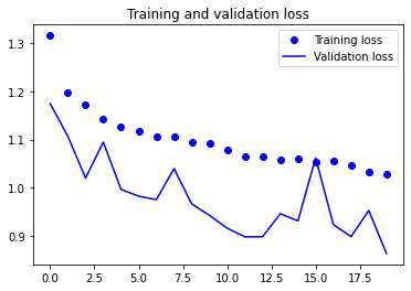
plt.plot(epochs, loss, 'bo', label='Training loss')
plt.plot(epochs, val_loss, 'b', label='Validation loss')
plt.title('Training and validation loss')
plt.legend()
plt.show()
'하루 30분 컴퓨터 비전 공부하기' 카테고리의 다른 글
| CV(8) Segmentation과 U-Net (0) | 2023.10.31 |
|---|---|
| CV(7) Object Detection과 R-CNN (0) | 2023.10.27 |
| CV(5) CNN 정복하기 GoogLeNet - 심화된 CNN 구조 (1) | 2023.10.26 |
| CV(2) CNN 기초 - Convolution, filter, padding (0) | 2023.10.25 |
| CV(4) CNN 기초 - pooling (0) | 2023.10.25 |


