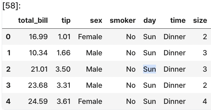
seaborn 패키지에서 제고하는 데이터를 가지고 내가 받을 수 있는 팁이 얼마인지 간단히 예측하는 모델을 설계해 보도록 하겠습니다.
먼저 데이터를 불러오도록 하겠습니다.
import seaborn as sns

tips = sns.load_dataset('tips')
tips.head()
먼저 string형태의 데이터를 원-핫 인코딩으로 변환하여 실수형 으로 바꿔주겠습니다. 데이터의 형태를 바꿔주는 이유는 수식에 넣어 계산 할것이기 때문입니다.
import pandas as pd
tips = pd.get_dummies(tips, columns = ['sex', 'smoker', 'day', 'time'])
tips.head()
# col의 순서 바꾸기
tips = tips[['total_bill', 'size', 'sex_Male', 'sex_Female', 'smoker_Yes', 'smoker_No',
             'day_Thur', 'day_Fri', 'day_Sat', 'day_Sun', 'time_Lunch', 'time_Dinner', 'tip']]
(1)에서와 달리 이번에는 12개의 x값이 있기 때문에 모델을 다음과 같이 설정할 수 있습니다.
y=w1x1+w2x2+w3x3+w4x4+w5x5+w6x6+w7x7+w8x8+w9x9+w10x10+w11x11+w12x12+b
선형회귀
: 종속 변수 y와 한 개 이상의 독립 변수 (또는 설명 변수) X와의 선형 상관 관계를 모델링하는 회귀분석 기법 (https://ko.wikipedia.org/wiki/%EC%84%A0%ED%98%95_%ED%9A%8C%EA%B7%80
즉, 선형방정식을 활용하여 모델을 설계하고 값을 예측하고 학습시키는 것을 말합니다.
- X, y 값 설정하기
X = tips[['total_bill', 'size', 'sex_Male', 'sex_Female', 'smoker_Yes', 'smoker_No',
          'day_Thur', 'day_Fri', 'day_Sat', 'day_Sun', 'time_Lunch', 'time_Dinner']].values
y = tips['tip'].values
- test데이터 셋과 train 데이터 셋 나누기
# sklearn의 train_test_split을 통해 train, test 데이터셋 나누기
from sklearn.model_selection import train_test_split

X_train, X_test, y_train, y_ test = train_test_split(X, y, test_size = 0.2, random_state= 42)
print(X_train.shape, y_train.shape)
print(X_test.shape, y_train.shape)train_test_split(X, y , test_size = , random_state = , shuffle = True, stratify = y)
- test_size : 테스트 세트의 크기를 지정, 기본값 0.25(25%)
- tarin_size : 훈련 세트의 크기를 지정, test_size와 배타적이므로 일반적으로 사용하지 않음
- random_state : 난수 생성기의 seed를 지정, 특정값을 설정하면 동일한 결과를 얻을 수 있음
- shuffle : 데이터를 섞을지 여부를 결정
- stratify : 분류 문제에서 클래스의 분포를 유지하기 위해 지정

- w와 b의 초기값 설정하기
import numpy as np
W = np.random.rand(12) # x가 12이기 때문
b = np.random.rand()

print(W)
print(b)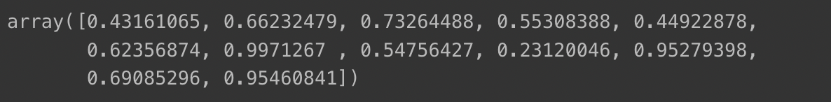

W에는 12개의 래덤한 값이 b에는 1개의 랜덤한 상수값이 할당되었습니다.
- 모델 구현
# 모델
def model(X, w, b):
	prediction = 0
	for i in range(12):
		prediction += x[:, i] * W[i]
		prediction += b
	return prediction

# MSE손실함수
def MSE(predict, y):
	mse = ((predict - y)**2).mean() # 두 값의 차이의 제곱의 평균
	return mse

def loss(X, W, b, y):
	prediction = model(X, W, b)
	L = MSE(prediction, y)
	return L

def gradient(X, W, b, y):
	# N은 데이터 포인트의 개수
	N = len(y)

	# y_pred준비
	y_pred = model(X, W, b)

	# gradiednt계산
	dW = 1/N * 2 * X.T.dot(y_pred -y)

	# b의 gradient 계산
	db = 2 * ( y_pred -y).mean()
	return dW, db


# 경사하강법으로 모델학습하기
LEARNING_RATE = 0.0001

losses = []

for i in range(1, 1001):
	dW, db = gradient(X_train, W, b, y_train)
	W -= LEARNING_RATE * dW
	b -= LEARNING_RATE * db
	L = loss(X_train, W, B, y_train)
	losses.append(L)
	if i % 10 == 0:
		print('Iteration %d : Loss %0.4f' %(i,L))

 import matplotlib.pyplot as plt
 plt.plot(losses)
 plt.show()
loss값이 잘 내려가는 것을 확인 할수있습니다.
그래프를 통해 시각화해봅시다.
prediciont = model(X_test, W, b)
mse = loss(X_test, W, b, y_test)

print(mse)

plt.scatter(X_test[:, 0], y_test)
plt.scatter(X_test[:, 0], prediction)
plt.show()
#데이터 준비하기
tips = sns.load_dataset("tips")
tips = pd.get_dummies(tips, columns=['sex', 'smoker', 'day', 'time'])
tips = tips[['total_bill', 'size', 'sex_Male', 'sex_Female', 'smoker_Yes', 'smoker_No',
             'day_Thur', 'day_Fri', 'day_Sat', 'day_Sun', 'time_Lunch', 'time_Dinner', 'tip']]
X = tips[['total_bill', 'size', 'sex_Male', 'sex_Female', 'smoker_Yes', 'smoker_No',
'day_Thur', 'day_Fri', 'day_Sat', 'day_Sun', 'time_Lunch', 'time_Dinner']].values
y = tips['tip'].valuestrain_test_split로 train, test데이터셋 설정하기
X_train, X_test, y_train, y_test = train_test_split(X, y, test_size=0.2, random_state=42)이제 sklearn안에 있는 모델을 가져다 쓰면 됩니다.
from sklearn.linear_model import LinearRegression
model = LinearRegression()

model.fit(X_train, y_train)
predictions = model.predict(X_test)
print(predictions)
from sklearn.metrics import mean_squared_error

mse = mean_squared_error(y_test, predictions)
print(mse)
'TIL(Today I Learned)' 카테고리의 다른 글
| likelihood와 머신러닝 (0) | 2023.09.12 |
|---|---|
| scikit-learn을 이용해 분류문제 해결하기 (0) | 2023.09.05 |
| 시계열 데이터 분석, 예측하기 (1) | 2023.08.31 |
| 데이터 분석 (0) | 2023.08.30 |
| 머신러닝 모델설계하기 기초(1) (0) | 2023.08.28 |


